

Parametric representations using polynomials are simply not powerful enough, because many curves (e.g., circles, ellipses and hyperbolas) can not be obtained this way. One way to overcome this shortcoming is to use homogeneous coordinates. For example, a curve in space (resp., plane) is represented with four (resp., three) functions rather than three (resp., two) as follows:
Space curve: F(u) = ( x(u), y(u), z(u), w(u) )where u is a parameter in some closed interval [a,b]. Converting this curve to their conventional form yields the following:
Plane curve : F(u) = ( x(u), y(u), w(u) )
Space curve: f(u) = ( x(u) / w(u), y(u) / w(u), z(u) / w(u) )Obviously, if w(u) = 1, a constant function, the homogeneous forms reduce to conventional forms.
Plane curve : f(u) = ( x(u) / w(u), y(u) / w(u) )
A parametric curve in homogeneous form is referred to as a rational curve. To make a distinction, we shall call a curve in polynomial form a polynomial curve.
Let the domain of u be the real line. Now, let u run from negative infinity to positive infinity. The values of x and y will both go to infinity, positive or negative. In other words, the curve described by the above parametric form contains at least one point at infinity. Since all points of a circle are in finite range, it is impossible to obtain a circle from the above parametric form. So, this shows a weakness of parametric form.
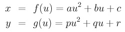
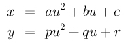
We can also reach this conclusion through calculation. Let us start with the following form:
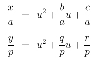
Assume a and p are both non-zero. Dividing the first and second equation by a and p, respectively, we have
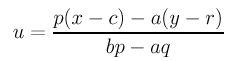
Now subtract the second from the first to eliminate the u2 term. Then, solving for u yields:
Finally, plugging this u back into the first equation (of the parametric form) gives
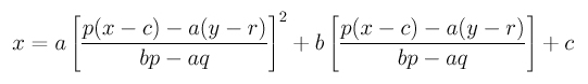
Clearing the denominators and rearranging terms gives
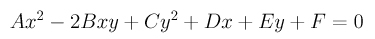
where
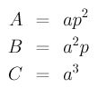
Recall that to determine the type of this quadric curve, we do not need the values of D, E and F. Since B2-A×C=0 (see Simple Curves and Surfaces for the details), this curve is a parabola. A problem in the Problems section addresses some of the minor flaws in the above calculation.
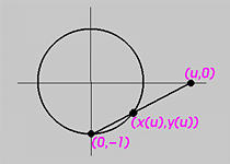
The above shows a circle with center at the origin and radius 1. Let u be a parameter for this circle. For convenience, we use the x-axis for the value of u, and, as a result, for any particular value of u there is a point (u,0) on the x-axis. Join a line between (u,0) and the south pole of the circle (0,-1). Since a line intersects a circle in two points, let the other point, which is not the south pole, be (x(u), y(u)). As u moves on the x-axis, its corresponding point moves on the circle. Any finite u has such a corresponding point. The infinite u corresponds to the south pole. On the other hand, any point on the circle that is not the south pole corresponds to a u on the x-axis.
The line joining the south pole and (u,0) is x = uy + u. The circle equation is x2 + y2 = 1. Plugging the line equation into the circle equation and solving for y yields two roots for y. One of them must be y = -1, since this line passes through the south pole. The other root is y = (1 - u2) / (1 + u2). Plugging this y into the line equation yields x = (2 u) / (1 + u2). Therefore, for each u, the corresponding point on the circle is
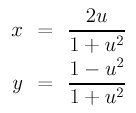
As a result, a circle has a rational parameterization. When u moves to infinity, x approaches 0 while y approaches -1 (use L'Hospital's rule).
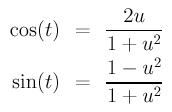
In fact, this computation tells us more. This circle has a trigonometric parametric form ( cos(t), sin(t) ), where t is in the range of 0 and 2PI. Therefore, a point on the circle can have two different representations, but their values are equal. That is, ( cos(t), sin(t) ) = ( (2 u) / (1 + u2), (1 - u2) / (1 + u2) ) for some u. Hence, trigonometric functions cos(t) and sin(t) can be parameterized as follows:
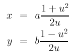
With a parameterization for cos(t) and sin(t) in hand, you can easily find a rational parameterization for an ellipse and a hyperbola. Let us do the hyperbola part and leave the ellipse as an exercise. A hyperbola in its normal form has an equation as follows:
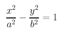
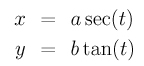
where a and b are the semi-major axis and semi-minor axis lengths. It is easy to verify that the following is a correct parameterization for the hyperbola:
The question is: given a curve in an implicit polynomial form, is it possible to find a parametric form, polynomial or rational, that describes the same curve? Unfortunately, the answer is negative. That is, there exists curves which do not have any polynomial or rational parametric forms (e.g., the elliptic curve y2 = x3 + ax + c). This is the result of uniformization theorems.
Due to this fact, implicit polynomials can describe more curves than polynomial and rational parametric forms. Why don't we use implicit polynomials? The reason is simple. Parametric curves are easy to use. While implicit polynomial curves are powerful and can describe more curves, many of its important properties are difficult to compute and implicit curves are in general difficult to use. We shall cover implicit curves and surfaces later.