Curve Global Interpolation

The simplest method of fitting a set of data points with a B-spline curve is the global interpolation method. The meaning of global will be clear later on this page.
Suppose we have n+1 data points D0, D1, ..., Dn and wish to fit them with a B-spline curve of degree p, where p <= n is an input. With the technique discussed in Parameter Selection and Knot Vector Generation, we can select a set of parameter values t0, t1, ..., tn. Note that the number of parameters is equal to the number of data points, because parameter tk corresponds to data point Dk. From these parameters, a knot vector of m + 1 knots is computed where m = n + p + 1. Thus, we have a knot vector and the degree p, the only missing part is a set of n+1 control points. Global interpolation is a simple way of finding these control points.
Global Curve Interpolation |
Suppose the desired interpolating B-spline curve of degree p is the following:
This B-spline curve has n + 1 unknown control points. Since parameter tk corresponds to data point Dk, plugging tk into the above equation yields the following:
Because there are n + 1 B-spline basis functions in the above equation (N0,p(u), N1,p(u), N2,p(u), ..., and Nn,p(u) and n +1 parameters (t0, t1, t2, .., and tn), plugging these tk's into the Ni,p(u)'s yields (n+1)2 values. Click here to learn how to compute these coefficients. These values can be organized into a (n+1)×(n+1) matrix N in which the k-th row contains the values of N0,p(u), N1,p(u), N2,p(u), ..., and Ni,p(u) evaluated at tk as shown below:
Let us also collect vectors Dk and Pi into two matrices D and P as follows:
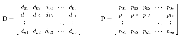
Here, data point Dk is a vector in s-dimensional space (i.e., Dk = [ dk1, ....., dks]) and appears on the k-th row of matrix D. Similarly, Pi is a vector in s-dimensional space (i.e., Pi = [ pi1, ....., pis]) and appears on the i-th row of matrix P. Note that in three-dimensional space, we have s = 3, and in a plane we have s = 2. Note also that D and P are both (n+1)×s matrices. Now, it is not difficult to verify that the relation of Dk's and ti's is transformed into the following simpler form:
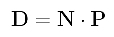
Since matrix D contains the input data points and matrix N are obtained by evaluating B-spline basis functions at the given parameters, D and N both are known and the only unknown is matrix P. Since the above is simply a system of linear equations with unknown P, solving for P yields the control points and the desired B-spline interpolation curve becomes available. Therefore, the interpolation problem is solved!
You might have something in doubt because matrices D and P are not column matrices as discussed in your numerical methods and linear algebra textbooks. This actually causes no problem at all. We can solve this system column by column. More precisely, let the i-th column of D and the i-the column of P be di and pi, respectively. From the above system of linear equations, we have the following:
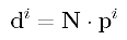
Then, solving for pi from N and di gives the i-th column of P. Do this for every i in the range of 0 and h, and we will have a complete P. Hence, all control points are computed. As you might have noticed, this is very inefficient. Fortunately, many numerical libraries provide us with a linear system solver that is capable of solving the equation D = N.P efficiently. Thus, fitting a B-spline curve to a set of n+1 data points is not very difficult. It boils down to the solution of a system of linear equations. The following algorithm summarizes the required steps:
Input: n+1 data points D0, ..... Dn and a degree p
Output: A B-spline curve of degree p that contains all data points in the given order
Algorithm:
Select a method for computing a set of n+1 parameters t0, ..., tn;
As a by-product, we also receive a knot vector U;
for i := 0 to n do
for j := 0 to n do
/* matrix N is available */
Evaluate Nj,p(ti) into row i and column j of matrix N;
for i := 0 to n do
Place data point Di on row i of matrix D;
/* matrix D is constructed */
Use a linear system solver to solve for P from D = N.P
Row i of P is control point Pi;
Control points P0, ..., Pn, knot vector U, and degree p determine an interpolating B-spline curve;
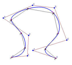
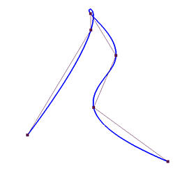
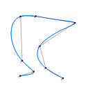
Figure (a) below is an example. There are 9 data points in black. The computed control points are in blue. The small blue dots on the interpolating curve are points corresponding to the knots which are computed using the chord length method. In this case, these "knot points" are quite close to the data points and the control polygon also follows the data polygon closely, although it is not always the case. In Figure (b) below, the data polygon and the control polygon are very different.
|
|
| (a) | (b) |
It is important to point out that matrix N is totally positive and banded with a semi-bandwidth less than p (i.e., Ni,p(tk) = 0 if |i - k| >= p) if the knots are computed by averaging consecutive p parameters. This was proved by de Boor in 1978. See Knot Vector Generation for the details. This means the system of linear equations obtained from the above algorithm can be solved using Gaussian elimination without pivoting.
In general, the impact of the selected parameters and knots cannot be predicted easily. However, we can safely say that if the chord length distribution is about the same, all four parameter selection methods should perform similarly. Moreover, the universal method should perform similar to the uniform method because the maximums of B-spline basis functions with uniform knots are distributed quite uniformly. Similarly, the centripetal method should work similar to the chord length method because the former is an extension to the latter. However, it is not always the case when the distribution of chord lengths change wildly.
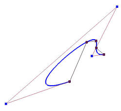
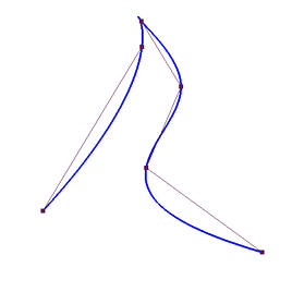
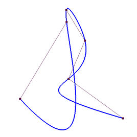
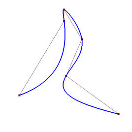
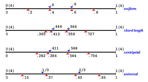
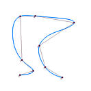
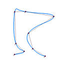
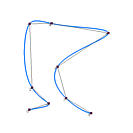
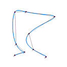
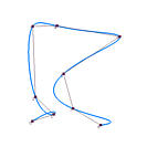
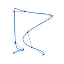
The following four curves are obtained using four parameter selection methods and the degree of the interpolating B-spline curve is 3. The uniform method generates a cusp, the chord length method forces the curve wiggle through data points wildly, the centripetal method resemblances the chord length method but performs better, and the universal method follows the data polygon closely (better than the uniform method) but produces a small loop.
|
|
| uniform | chord length |
|
|
| centripetal | universal |
How about the relation between parameters and knots? The following diagram shows the parameters and knots of all four methods. As you can see, the parameters and knots obtained from the universal method is more evenly distributed than those of the chord length method and the centripetal method. Moreover, the parameters and knots obtained from the centripetal method stretch the shorter (resp, longer) chords longer (resp., shorter) and hence are more evenly distributed. Therefore, the longer curve segments obtained by the chord length method become shorter in the centripetal method and the curve does not wiggle wildly through data points.
The impact of degree to the shape of the interpolating B-spline curve is also difficult to predict. One can easily observe, from the following images, that the uniformly spaced method and universal method usually follow long chords very well; however, they have problems with short chords. Because the parameters are equally or almost equally spaced, the interpolating curves have to stretch a little longer for shorter chords. As a result, we see peaks and loops. This situation gets worse with higher degree curves because higher degree curves provide more freedom to wiggle.
| |
Uniform | Chord Length | Centripetal | Universal |
| Deg 2 | 
|
|

|
|
| Deg 3 | 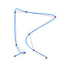
|

|
|

|
| Deg 4 | 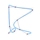
|

|
|

|
| Deg 5 | 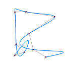
|
|
|
|
As for the chord length method, the above figures show that it does not work very well for longer chords, especially those followed or preceded by a number of shorter chords, for which big bulges may occur. There is no significant impact of degree on the shape of the interpolating curves shown above. Since the centripetal method is an extension to the chord length method, they share the same characteristics. However, since the centripetal method has a tendency to even out the distance between two adjacent parameters, it also shares the same characteristics of the uniform and universal methods. For example, the generated interpolating curves follow longer chords closely and loops may occur for shorter chords when degree increases. In fact, results above show that the centripetal method and the universal method perform similarly.
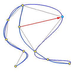
This interpolation method is global even with the use of B-spline curves which satisfy the local modification property, because changing the position of a single data point changes the shape of the interpolating curve completely. In the following figure, those yellow dots are data points and one of them is moved to its new position, marked in light blue and indicated with a red arrow. These nine data points are fit with a B-spline curve of degree 4 using the centripetal method. As you can see, the resulting curve (in blue) and the original curve have eight data points identical, and the eight curve segments are all different. Therefore, changing the position of s single data point changes the shape of the interpolating curve globally!