
Knot insertion is one of the several fundamental geometric algorithms that permit to modify the defining parameters of a surface without changing its shape. It is based on the knot insertion algorithm for B-spline and NURBS curves. Click here to review the details of knot insertion.
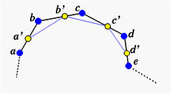
Due to the fundamental identity (i.e., m = n + p + 1, where m+1, n+1, and p are the number of knots, the number of control points, and the degree of a B-spline or a NURBS curve), adding one knot requires adding one or control point. In general, if the curve degree is p, then p+1 consecutive control points involve in the knot insertion process by corner cutting. In the following figure, suppose the curve degree is 4. Then, we need 5 consecutive control points, say a, b, c, d and e. A knot insertion algorithm will pick one point from each of these four segments, say a' from segment ab, b' from segment bc, c' from segment cd, and d' from segment de. The new control polygon includes all control points before a, all control points after e, and control points a, a', b', c', d' and e. In effect, the corners at b, c and d are cut.
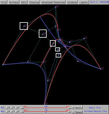
For a B-spline or a NURBS surface, one can insert a new knot in the u- or the v-direction. If the new knot is inserted in the u-direction (resp., v-direction), the above knot insertion process will be applied to all sets of control points that define isoparametric curves in the same direction. Let us use the surface in the default scene two as an example. Since we need to see the impact on control points, we choose to display knot curves without the surface. The surface in default scene two is a NURBS surface with 4 rows and 5 columns and the degrees in the u- and v- directions are 2 and 3, respectively.
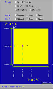
To insert a new knot 0.25 in the u-direction, we need to move the uv-indicator so that its u value is 0.25. Since the degree in the u-direction is 2, three consecutive control points involve in the knot insertion process.
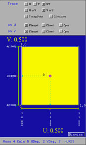
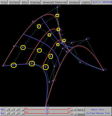
Now, select Advanced Features, followed by Knot Insertion, followed by on U. Then, the u value of the current position of the uv-indicator is inserted as a new knot into the knot vector in the u-direction. The right figure below shows this new knot. After corner cutting, on each row an existing control point (those marked with white rectangles above) is removed and replaced with two new control points, which are marked in yellow rectangles below. Also note that a new knot curve corresponding to the new knot u = 0.25 is shown.
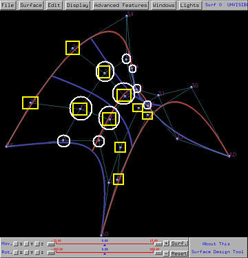
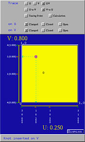
Let us insert v = 0.8 into the knot vector in the v-direction. Move the uv-indicator until its v value is equal to 0.80. Then, select Advanced Features, followed by Knot Insertion, followed by on V. Since the surface is of degree 3 in the v-direction, four control points in each "column" involve in the knot insertion process, and two of them will be cut and replaced with three new control points. The control points that will be cut are shown in white circles in the above figure. After the new knot is inserted, we have the following (left) figure in which the new control points are shown in yellow circles. Note also that the new knot v = 0.8 is shown in the Tracing Window, and the new knot curve is shown in red.
As mentioned earlier, knot insertion does not change the shape of the give surface (this can be seen in the above three figures); but, the number of control points is increased.
If the new knot value is equal to an existing one, the new (and of course the existing) one becomes a multiple knot. Otherwise, the new knot is a simple knot. Note that increasing the multiplicity of a knot decreases its continuity on the surface.