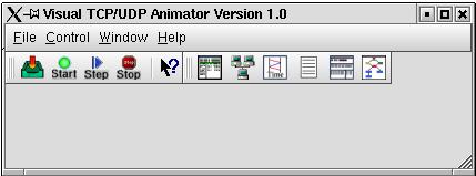
Figure 1: VTA main frame window
Here are some screen shots that show VTA in action.
VTA displays data in any of six views. The stream of data displayed in these views begins from a user-specified source. This stream then passes through an optional filter, and then feeds into the selected views. Figure 1 shows the VTA main frame window.
Figure 1: VTA main frame window
Figure 2 is the first window of the user wizard, which will guide users through the input data specification process. A user may select one from among the options Disk File, All Realtime Traffic, Current Active Sockets, or Specific Application as the initial source of the packet stream which feeds into the VTA views.
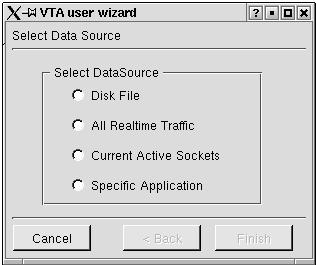
Figure 2: VTA Data Specification Window
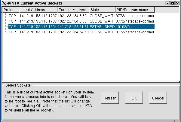
Figure 3: VTA Active Socket Window
Whichever of these sources is selected, a subsequent filter can optionally be applied to the stream prior to its display by VTA. Users may optionally specify a filter of source or destination IP address and port for these packets. Figure 4 shows the socket filter specification window.
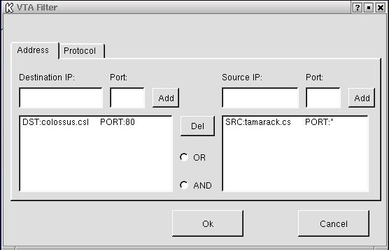
Figure 4: VTA Socket Filter Speicification Window
Once the input packet stream has been configured, any of six views can be selected for display of the stream. Capture and display begins upon selecting Start from the main frame window (shown in Figure 1), and continues until Stop is selected or no additional data is available. A step mode, in which a single packet is displayed for each step, is also available.
Figure 5 shows the packet list view. A summary
line
is displayed for each captured packet. The summary line
contains:
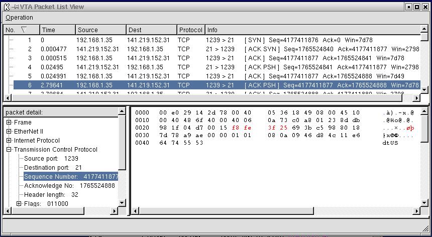
Figure 5: VTA Packet List View
Figure 6 shows the connection packet view. A summary line appears for each TCP connection. The summary line contains the source and destination addresses (<IP address,port>). Selecting a particular connection displays a summary line, similar to that of the packet view, for each packet that has been sent or received, by the host, along the connection. Selecting the summary line for a particular packet displays the data contained in that packet in binary and ASCII format.
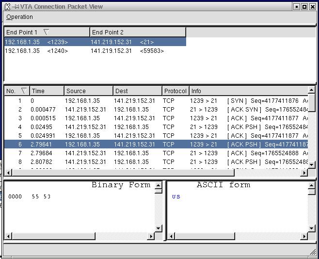
Figure 6: VTA Connection Packet View
Figure 7 shows the Connection Reconstruction
View. This view attempts to depict data transmitted along the connection
as a conversation between the communication endpoints. A summary line is
displayed for each TCP connection. Selecting a single connection
displays the data, in ASCII format, that has flowed across the connection.
The bottom two subwindows depict reconstructed TCP data sent by each endpoint.
During the reconstruction, duplicates are removed, packets are reordered
according to their sequence number. Different text colors denote the direction
of the data transmission. For example, data transmitted from the
VTA host to receiver always appears in a single color that is different
from the single color used to depict data received by the VTA host.
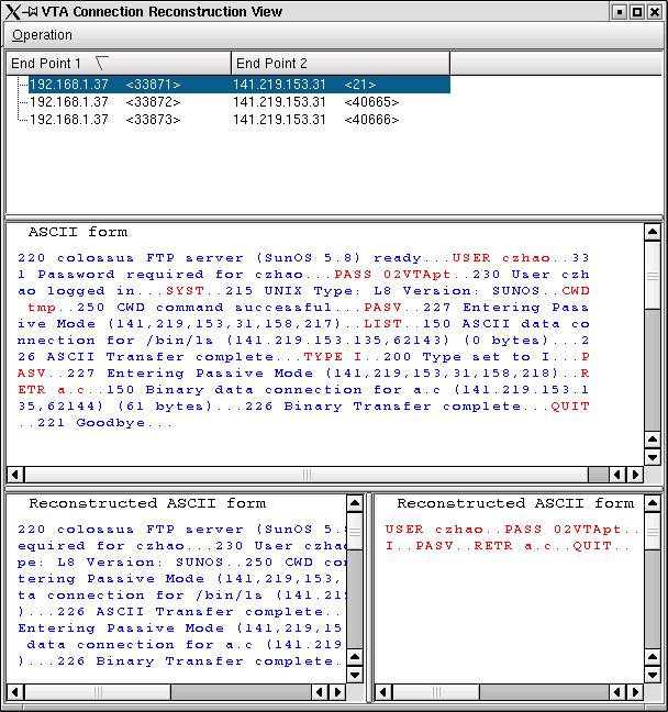
Figure 7: VTA Connection Reconstruction View
Figure 8 shows the machine distribution view. It displays
an undirected graph where edges correspond to source/destination pairs
in a captured packet and nodes correspond to IP addresses. For each
node, an IP address and number of packets sent and received is displayed.
In order to display the machine distribtion, an automatic layout algorithm
based on a spring-embedder model is used. Attractive forces are assigned
on all links and repulsive forces are assigned between nodes. Iteration
is used in an attempt to acheive balance. This technique can produce
reasonable layouts of many networks, but may not produce satisfactory results
of complicated networks. As a remedy, VTA allows the user to graphically
adjust the resulting layout.
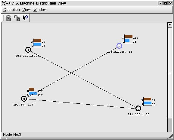
Figure 8: VTA Machine Distribution View
Figure 9 shows the timeline view. In the timeline view, an axis appears for each new socket (<IP,port> pair). Each sent or received packet results in an arrow between the axes corresponding to the source and destination. Both UDP and TCP communications are displayed. (If the transmission is based on UDP, the arrow appears dashed; if the transmission is based on TCP the arrow appears solid.)
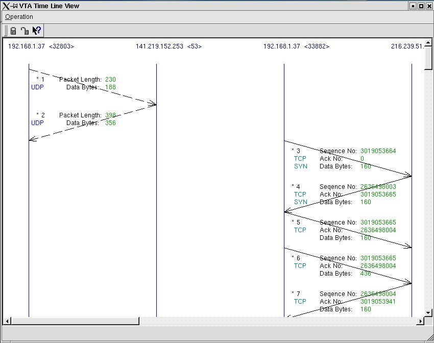
Figure 9: VTA Timeline View
The TCP Staus view is shown in Figure 10. This view depicts the state of a TCP connection within the protcol state transition diagram. Different colors, red or green, mark the state in which the two connection endpoints currently reside. A third color marks states through which the connection has passed.
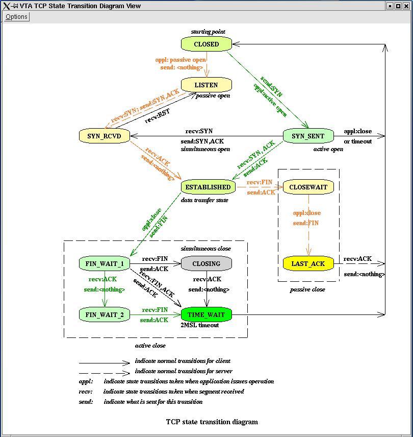
Figure 10: VTA TCP State Transistion Diagram View